Cap a Möbius Strip and You Get the Projective Plane: I Implemented Boy's Surface and Exactly One Triple Point Appeared

A Möbius strip has an edge. On an ordinary band the edge comes in two pieces, top and bottom. But run your finger along one edge of a Möbius strip and at some point you find yourself traveling along what should have been the other edge, returning to the start only after going around twice. The edge is a single closed loop. So what happens if you take that one loop and cap it with a disk?

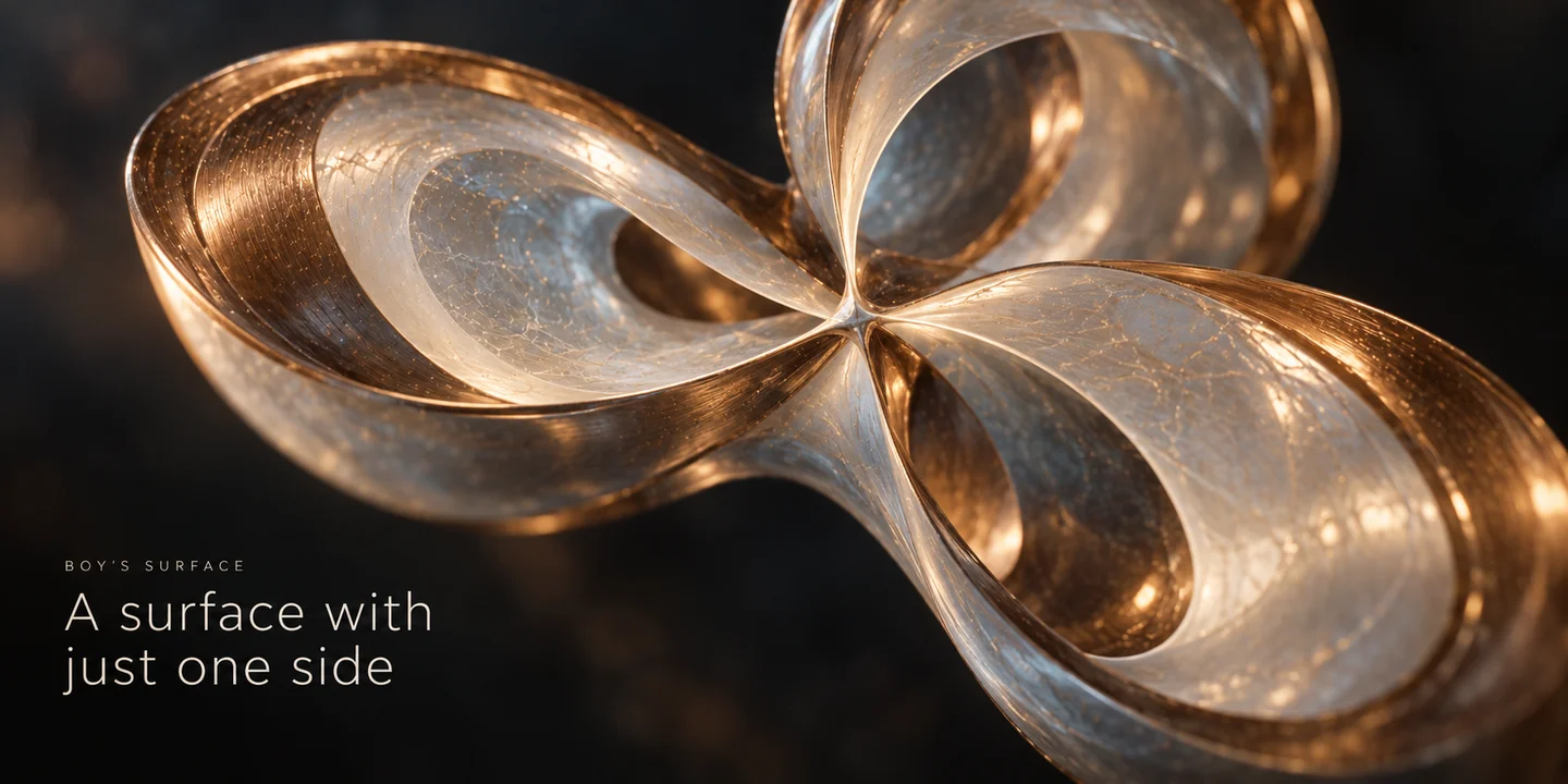
What you get is a closed surface with no edge, and one with no distinction between front and back — the surface called the real projective plane. It has an inconvenient property, though. Unlike the sphere or the torus, it cannot be placed in 3-dimensional space without self-intersection. Same situation as the Klein bottle. One of the shapes you get when you force it into 3D anyway is Boy’s surface, discovered in 1901.

Words alone are not convincing, so as usual I built the whole thing in code and checked it with numbers.

Red is the “disk,” blue is the “Möbius band,” and the black curve is the seam between them. In other words, the figure above is exactly the paper-craft from the opening — capping a Möbius strip with a disk — carried out in 3D. Try clicking the legend to show only the red, or only the blue.

The full code for the experiment is on GitHub.

Building Boy’s surface: the gluing was baked into the formula

Boy’s surface has a surprisingly compact parametrization due to Bryant and Kusner. For a complex number $w$ on the unit disk ($|w| \le 1$), set

$$g_1 = -\frac{3}{2}\,\mathrm{Im}\!\left[\frac{w(1-w^4)}{w^6+\sqrt{5}\,w^3-1}\right],\quad g_2 = -\frac{3}{2}\,\mathrm{Re}\!\left[\frac{w(1+w^4)}{w^6+\sqrt{5}\,w^3-1}\right],\quad g_3 = \mathrm{Im}\!\left[\frac{1+w^6}{w^6+\sqrt{5}\,w^3-1}\right]-\frac{1}{2}$$

and then take $(x,y,z) = (g_1,g_2,g_3)/(g_1^2+g_2^2+g_3^2)$. That’s all. You don’t need to follow what the formula is doing. The only thing worth holding onto is that the input is a single unit disk — that matters later. Why there is a $\sqrt{5}$ in the denominator, I don’t know either. It fits in a few dozen lines of numpy.

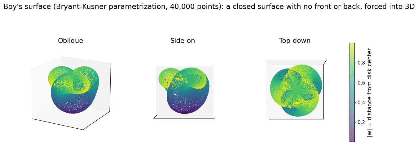
The textbook definition of the real projective plane is “a disk with antipodal points on its boundary glued together.” The first thing that struck me on implementing it was that this gluing is already built into the formula. Measuring the distance between $f(w)$ and $f(-w)$ at 4001 points:

• On the boundary $|w|=1$: maximum 8.5×10⁻¹⁶. The same point to machine precision — the antipodal boundary points are indeed glued
• In the interior ($|w|=0.5$): minimum 1.71. Interior points are not glued

I checked the topology on a mesh as well, using the Euler characteristic $\chi = V - E + F$. It’s just an integer — count vertices, subtract edges, add faces — but it doesn’t change no matter how you bend or stretch the surface. A fingerprint for surfaces. Counting directly from the triangulation:

Surface	Construction	$V-E+F$	Theory
Disk	edge not glued	1	1
Annulus	band, edges not glued	0	0
Möbius band	antipodal points of the annulus’s outer edge glued	0	0
Real projective plane	antipodal points of the disk’s edge glued	1	1
Sphere (control)	—	2	2

The gluing checks out arithmetically too: $\chi(\text{Möbius}) + \chi(\text{disk}) - \chi(\text{circle}) = 0 + 1 - 0 = 1 = \chi(\text{projective plane})$. The addition implied by the opening paper-craft actually holds.

Confirming “Möbius band + disk” in coordinates

The Euler characteristic is circumstantial evidence, though. To claim outright that this is a capped Möbius strip, it’s faster to take it apart and show it.

Cut the parameter disk in two with a circle of radius 0.65. The inside is an ordinary disk. The outer ring-shaped piece — since antipodal points on the edge $|w|=1$ are glued — should be a single band, connected to its own far side at the middle of its width.

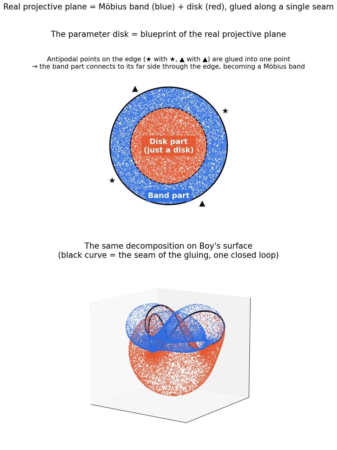
I re-parametrized the outer piece in the standard Möbius coordinates $(\sigma, t)$ ($\sigma$ the position along the band, $t$ the width direction) and ran four checks.

1. Is the band’s center line continuous across the edge? The center line ($t=0$) corresponds to the disk’s edge $|w|=1$. Taking two points straddling the edge, the 3D distance between them shrinks as 2.0×10⁻² → 2.0×10⁻³ → 2.0×10⁻⁴ as the parameter gap $\varepsilon$ goes 10⁻²→10⁻³→10⁻⁴ — linear convergence to zero. There is no step at the seam
2. Does the width flip after one lap? Going once around the band ($\sigma: 0 \to \pi$) and coming back, the two ends match only when the width direction is reversed (maximum distance 2.5×10⁻⁹). Matched without reversing, the gap is 1.33. So this band carries exactly one twist — it is a Möbius band
3. Does the normal flip over? Tracking the normal vector continuously along the center line, by the time we return to essentially the same point (distance 3.5×10⁻⁴) the inner product of the normals is −1.000000. It comes back inverted. As a control, a loop that doesn’t pass through the gluing (the circle $|w|=0.5$) gives +1.000000
4. Is the band’s edge the same circle as the disk’s edge? Sampling the two at unrelated angles and measuring nearest-neighbor distance gives a maximum of 6.2×10⁻⁴, below the sampling interval (1.2×10⁻³). A control with the radius shifted by just 0.05 gives 0.31. Both lie on the same single closed curve

Every part of the textbook one-liner — “glue a disk to the edge of a Möbius strip and you get the projective plane” — checks out in coordinates and distances. Where the Klein bottle is “two Möbius bands glued along their edges,” the projective plane is “one Möbius band capped with a disk.” Siblings in the Möbius family.

The self-intersection turned out to be a three-bladed propeller

We forced something into 3D that doesn’t fit there, so somewhere the surface must be passing through itself. Searching a 170,000-point cloud for pairs that are “close in 3D but far apart on the projective plane,” 16,601 of the 980,000 neighbor pairs came back as evidence of self-intersection. Their distribution is the interesting part.

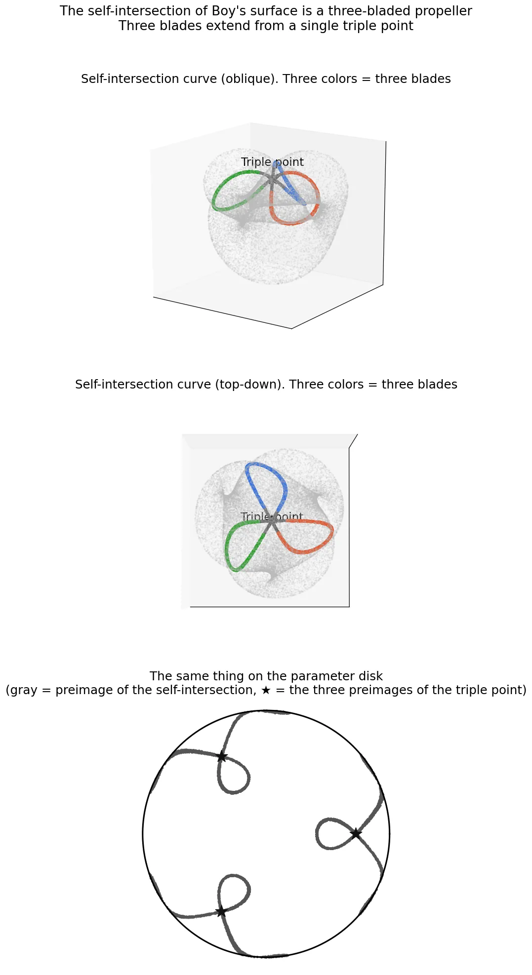
The self-intersection curve consists of three “blades” meeting at a single point. That look is why it’s called a three-bladed propeller. The structure the numbers gave:

• There is exactly one triple point (a point where three sheets overlap at once). Detected at $(-0.0008, -0.0008, -0.0015)$, a distance of 0.0019 from the origin
• Remove a neighborhood of the triple point and the self-intersection curve splits into exactly three arcs (5050 / 4583 / 4361 detected points)
• Include the triple point and the whole thing is connected. One triple point, three blades

The triple point landing on the origin is no accident. The denominator $w^6+\sqrt{5}w^3-1$ in the Bryant-Kusner formula vanishes at three points inside the disk (radius $((3-\sqrt{5})/2)^{1/3} = 0.72556$, angles 0°, 120°, 240°). There $g$ blows up, and the final inversion $g/|g|^2$ sends all three to the origin together. A singularity of the formula is a prediction about the geometry. Measuring the preimages of the detected triple point gives $|w| = 0.7259 \pm 0.0043$ and an angular deviation from theory of $+0.10° \pm 0.35°$. Exactly where it was predicted to be.

Incidentally, there is deep theory about how many self-intersections you need when forcing a closed surface into 3D: for the projective plane you are stuck with an odd number of triple points no matter what you do (Banchoff’s theorem). One is the minimum.

Before dimensionality reduction: do not start from 3D

Now for the main theme of this series, dimensionality reduction. The Swiss roll could be unrolled, the knot could be untied, and the Möbius strip balanced its books by crushing its own width. What happens to the projective plane, which has no front or back and is also closed?

There was a pitfall right at the start. Using the 3D point cloud of Boy’s surface directly, 5.5% of the kNN graph edges become shortcuts to a different sheet across the self-intersection (15.1% of points carry at least one such false edge; the control sphere, which has no self-intersection, gives 0.0%). The self-intersection is only a curve of measure zero, and yet the moment you sample at finite density it contaminates the graph. That would make this an experiment about a broken graph, not about the projective plane.

So I built a genuine, self-intersection-free projective plane in 6 dimensions. It’s a classical construction called the Veronese embedding: map a point on the sphere to

$$(x,y,z) \mapsto (x^2,\ y^2,\ z^2,\ \sqrt{2}xy,\ \sqrt{2}yz,\ \sqrt{2}zx)$$

Since $p$ and $-p$ land on the same point, antipodal identification comes for free, and distinct points never collide. Impossible in 3D, but raise the dimension and the projective plane can exist without self-intersection — the same idea as putting the Klein bottle in 4D.

I ran this alongside a sphere (an orientable closed surface) and a disk (just a flat patch) through four methods down to 2D.

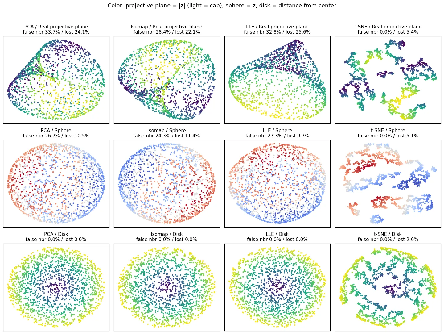
I measured two metrics. The false-neighbor rate is the fraction of pairs that are adjacent in the flattened picture but far apart on the actual surface — in moving-house terms, the rate at which total strangers move in next door. The lost-neighbor rate is the opposite: the fraction of pairs that were genuinely neighbors but got scattered apart in the flattening. Losing your neighbors in the move.

• Disk: essentially 0% / 0% for every method. An open patch flattens without trouble
• Sphere: 24–27% false, 10–11% lost. A closed surface has to either overlap something or tear
• Real projective plane: 28–34% false, 22–26% lost. Worse than the sphere, with roughly double the lost-neighbor rate

And once again there was a trap in the metrics. t-SNE’s false-neighbor rate is 0.0% on every dataset. On the numbers alone it wins outright, but look at the picture and it is simply tearing the cloud into small fragments and arranging them. It avoids manufacturing fake neighborhoods by destroying the real ones. (The lost-neighbor rate still comes out low, around 5%, because neighborhoods survive inside each fragment.) That makes this the fourth time in this series that a single metric has failed to notice structural destruction.

A strip made by twisting and a strip made by gluing should have been “the same”

This is the experiment that surprised me most.

In the previous article I made a Möbius strip by twisting a band and placing it in 3D. If this article’s construction of the projective plane is right, then a Möbius band should also be constructible by gluing antipodal points of a cylinder — with no twist term anywhere in the formula. Topologically the very same Möbius band. So will Isomap give the same result on both?

My first attempt actually failed: I tried it on the equatorial band of a round sphere, and because that band is barrel-shaped, even the control annulus refused to flatten cleanly, so nothing was comparable. To remove the effect of curvature I based all three conditions on a flat cylinder of the same dimensions as last time: “unglued band / twisted band (the previous construction) / glued band (antipodal identification).”

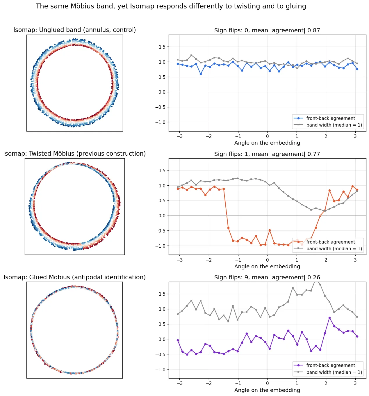
All three behaved differently.

• Unglued band (control): zero flips, front-back agreement 0.87. Nothing happens
• Twisted Möbius: reproduces the previous result. Front and back flip somewhere along the loop, and at the flip position the width is pinched to 15% of its median. A “local pinch” strategy that concentrates the distortion in one place
• Glued Möbius: unexpected. Neither a flip nor a pinch was observable. Instead, the width of the band itself was crushed to 3% of its true value all the way around. The ring is very nearly a single thread

The same manifold, and yet the algorithm changed how it lies. Last time I wrote that the options when facing an impossible demand are “tear / overlap / crush,” but it turns out “crush” itself comes in two styles: press it all into one point, or spread the burden thinly over everyone.

Why the change? The plausible explanation is this. The glued band has $(\sigma, t) \mapsto (\sigma, -t)$ — folding the band over at its center line — as a symmetry that preserves distances exactly (this follows necessarily from antipodal identification). A spectral method like Isomap (build a matrix of pairwise distances, take coordinates from its eigenvectors) sees only the distance matrix, so it has no reason to break that symmetry, and respecting the symmetry while dropping to 2D leaves the width direction nowhere to go. The band twisted into 3D, by contrast, has that symmetry slightly broken already by the act of placing it (at each point of the band, the local stretching on the outer and inner side differs according to the phase of the twist). That is why it can choose where to pinch. Consistent with this reading, the width crush reproduces under changes to the neighbor count $k$ and the sample size — while t-SNE, which is not a spectral method,

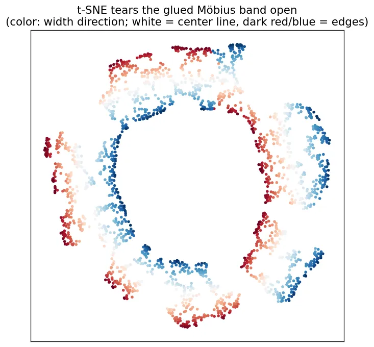
— threw the symmetry away entirely. It keeps the ring of the center line and shreds the edges into fragments arranged around the outside. The spectral method dies for the symmetry; the stochastic method kicks it aside. A contrast you won’t find in a textbook.

Bonus: an algorithm that decides “non-orientable”

So far I’ve looked at the absence of front and back by eye and through embeddings. Finally, I tried deciding orientability itself directly from the point cloud. It’s an application of the “propagate orientation through the neighbor graph” idea, passing the orientation of each point’s local tangent plane from neighbor to neighbor and counting whether it can be made consistent, as the number of connected components of the “orientation double cover.” In theory, an orientable surface gives two components — a front team and a back team — while a non-orientable one connects into a single component.

Point cloud	Components of the double cover	Verdict
Disk	2	Orientable
Sphere	2	Orientable
Unglued band (annulus)	2	Orientable
Twisted Möbius	1	Non-orientable
Glued Möbius	1	Non-orientable
Real projective plane (6D)	1	Non-orientable

All six match theory. Whether the embedding dimension is 3 or 6, whether the construction is a twist or a gluing, it names the topology correctly. You may not be able to draw the absence of front and back, but you can compute it.

What surprised me when I actually built it

The biggest takeaway was learning that traces of how you built a manifold survive into the algorithm’s output, even when the manifold is “the same.” The twisted band and the glued band are topologically identical and should be metrically near-identical, yet a slight difference in symmetry separated “pinch one point” from “crush the whole circumference.” Invisible symmetries introduced by how you preprocess or generate data can qualitatively change the behavior of downstream algorithms — I suspect that rings a bell well beyond manifold learning.

The other one: the “ugly part” of the formula was the crux of the geometry. The $\sqrt{5}$ and the sixth-degree term in the denominator weren’t decoration; their three zeros were exactly where the triple point lives. Until I implemented it, I thought that denominator was just a magic constant.

What this experiment cannot say

• “Exactly one” and “exactly three” hold only within the resolution of the detection. This is a cross-check that counted the triple point via 170,000-point sampling and neighbor search, not a proof. A numerical experiment cannot rule out finer structure slipping through the mesh of the detector. (Banchoff’s theorem guaranteeing an odd number is what lets me be comfortable reading it as one.)
• “Spectral methods can’t break the symmetry, so the whole circumference collapses” is an interpretation consistent with the observation, not a proof. The experiment that would settle it — a glued band with only the fold symmetry artificially broken, to see whether the crush turns into a pinch — I did not run.
• Numbers like 28–34% and 3% are not constants of these surfaces. They are experimental values depending on sample size and neighbor count, and they only mean something as comparisons between methods and between surfaces at identical settings.
• Whether “crush the whole circumference” is a property of spectral methods in general, I don’t know. I only tried Isomap and t-SNE; whether LLE or Laplacian eigenmaps choose the same lie is untested.

Capping something turned out to be a much heavier operation than I thought

Glue one disk onto a Möbius strip. As paper-craft that is the whole operation, and the resulting surface is evicted from 3-dimensional space, self-intersects however you place it, and is stuck carrying at least one triple point. A shape that lived peacefully in 3D as long as it had an edge loses its home the moment it closes up.

Even so, that homelessness was measurable end to end. The gluing mismatch is zero to machine precision, the normal returning after one lap has inner product −1.000000, and the address of the triple point was written into the denominator of the formula before anything was glued at all. Checking a single textbook line — “cap a Möbius band with a disk and you get the projective plane” — from end to end in coordinates and distances is the entirety of what I did here.

And on the flattened picture, the algorithm pays the price for that line. What cost one narrow pinch last time cost an entire circumference of crushing this time. Even within “placing something that cannot be placed,” the shape of the lie changes with how you built it. That choice — concentrate the sacrifice in one place, or spread it thinly over the whole — long predates the invention of dimensionality reduction. The tesseract’s shadow showed orthographic and perspective projection making the very same choice.