Measuring a Percolation Phase Transition: 1.5 Percentage Points Take the Spanning Probability From 0% to 100%

Take a square lattice and let each cell be “open” independently with probability $p$. Open cells that touch each other are connected. Is there a path of open cells running all the way from the top edge to the bottom edge? That question is called percolation. Whether hot water soaks through coffee grounds, whether a wildfire burns clear across a forest, whether a rumor makes it through a network — they all share this skeleton.

The interesting part starts here. Theory says 2D site percolation has a critical probability $p_c \approx 0.5927$: below it, the spanning probability is 0 (on an infinite lattice), above it, 1. Somewhere between 0.59 and 0.60 stands a cliff separating a world that doesn’t connect from a world that does.

The probability moves smoothly, and the outcome moves discontinuously. It’s the same shape as grokking — nothing happens for tens of thousands of steps and then suddenly the model gets it — an observable that jumps while the parameter you’re turning moves continuously. Is it really that abrupt? And can you see the cliff on a finite lattice at all? I measured it with numpy and scipy.

The full code for the experiment is on GitHub.

Experimental design

The task is simple, and the core of the implementation is about ten lines.

1. Build an $L \times L$ field of uniform random numbers $r$ and call a cell occupied when $r < p$
2. Detect all 4-neighbor connected clusters at once with scipy.ndimage.label
3. Declare “spanning” when the top row and the bottom row share a cluster label

I swept the occupation probability $p$ from $0.50$ to $0.70$ in steps of 0.005 and measured the spanning probability and the largest cluster size at each of $L = 64, 128, 256, 512, 1024$ (1000 trials at $L=64$, down to 80 at $L=1024$). On top of that, for each random field I found $p_{\mathrm{span}}$, the occupation probability at which that particular field first spans, by bisection. For a fixed random field, raising $p$ only ever adds occupied cells, so the spanning threshold can be pinned down to a precision of $10^{-4}$ by bisection. The distribution of $p_{\mathrm{span}}$ tells you both where the transition sits and how blunt it is.

First, watch it span

Here is what happens when you raise $p$ gradually on a single random field. Clusters are colored individually, a merged cluster inherits the color of whichever core formed first, and the cluster that spans top to bottom lights up yellow.

What was a scattering of small islands at $p=0.50$ starts merging like an avalanche from about 0.58, and on this particular field it spanned the screen at $p=0.595$. What matters here is not the newly placed cells themselves. The last 0.5% of cells act as bridges between continents that had already grown.

Lining up the landscape below, at, and above the transition on a larger lattice ($L=512$) looks like this.

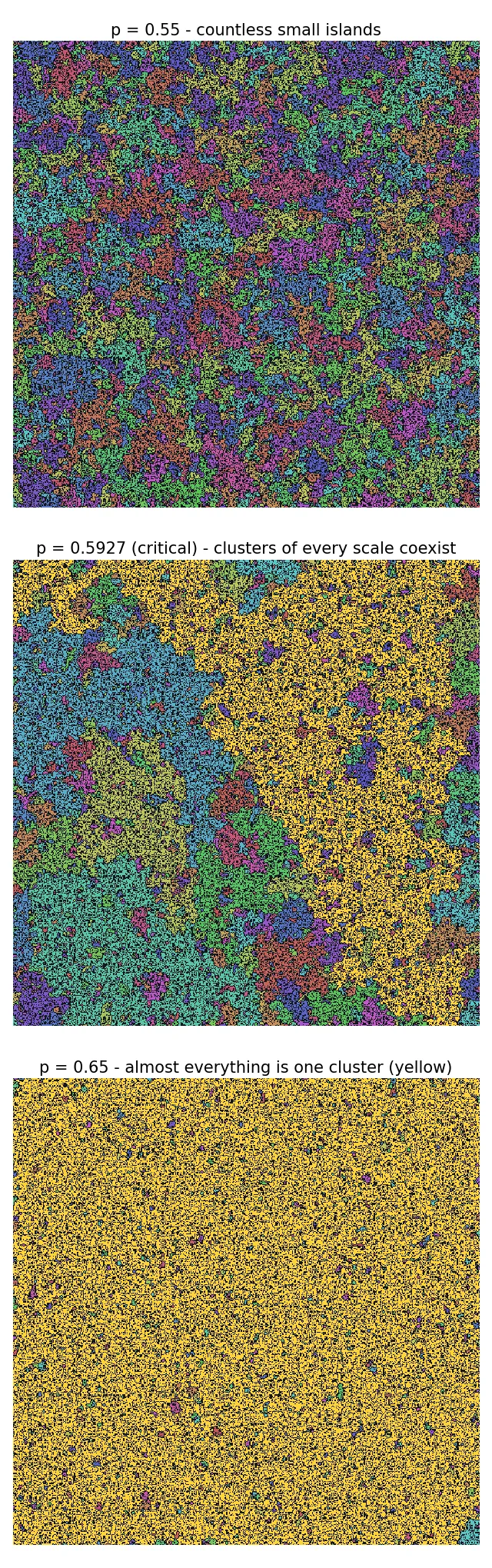
Only the landscape at the critical point is qualitatively different. Below it is “nothing but small islands,” above it is “almost one color,” while at the critical point clusters of every scale exist simultaneously. I’ll pin that “every scale” down quantitatively later, as a power law.

Result 1: the bigger the lattice, the more the transition becomes a cliff

The family of spanning-probability curves is the main result of this experiment.

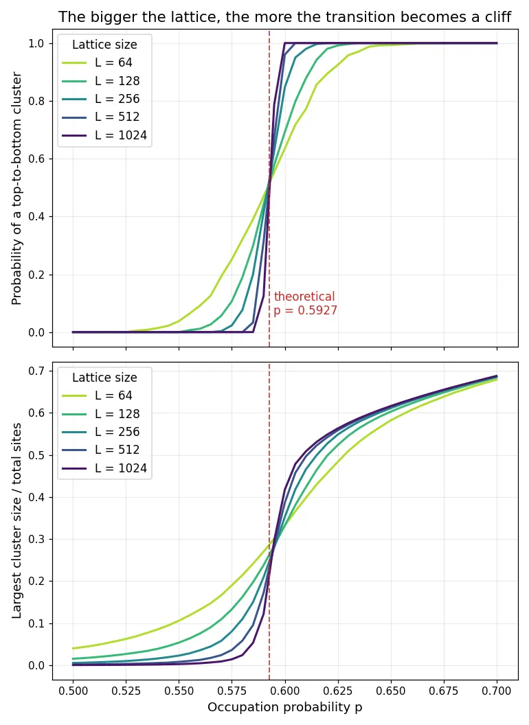
The transition at $L=64$ is gentle: even at $p=0.55$ it spans 3.8% of the time, and even at $p=0.65$ it fails to span 0.7% of the time. At $L=1024$, though:

Occupation p	0.585	0.590	0.595	0.600
Spanning probability (L=1024)	0.000	0.125	0.787	1.000

While the occupation probability moves a mere 1.5 percentage points, from 0.585 to 0.600, the spanning probability jumps from 0% to 100%. All 80 trials fail to span at 0.585, and all 80 span at 0.600. The largest cluster tells the same story: at $L=1024$ and $p=0.58$ the largest cluster is only 2.4% of the lattice, and at 0.60 a single cluster holds 41.7% of it.

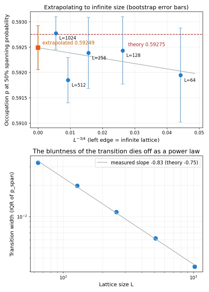
How the bluntness disappears can be measured by the spread (interquartile range) of the $p_{\mathrm{span}}$ distribution.

L	Transition width (IQR)	p at 50% spanning
64	0.0328	0.5919
128	0.0197	0.5924
256	0.0111	0.5924
512	0.0062	0.5918
1024	0.0033	0.5928

Going from $L=64$ to $L=1024$, a factor of 16, shrinks the transition width from 0.0328 to 0.0033 — exactly a factor of ten. The slope on the log-log plot is $-0.83$. Theory says the width should shrink as $L^{-1/\nu} = L^{-0.75}$ using the correlation-length exponent $\nu = 4/3$, so the sign and rough size of the slope agree, with a small discrepancy I’ll come back to. Because the shrinkage is a power law, the width never actually reaches zero no matter how large you go — but it heads there reliably. The textbook line “the transition is only truly discontinuous on an infinite lattice” shows up in front of you as a measured curve steepening into a cliff.

Result 2: the measured critical point is 0.5925 ± 0.0004

The occupation probability at which spanning hits 50% barely moves with lattice size, sitting around 0.592 at every size. Extrapolating to an infinite lattice with finite-size scaling ($p_{1/2}(L) = p_c + aL^{-3/4}$):

$p_c = 0.59249 \pm 0.00043$

The established numerical estimate $p_c \approx 0.59275$ falls neatly inside the error bar — within 1σ, off by 0.0003. Reading the $L=1024$ median directly gives 0.59277, a mere 0.00002 from that estimate, but that agreement is an order of magnitude finer than the uncertainty (±0.0003), so honestly it’s luck. Redraw the random numbers and that digit moves.

Result 3: the power law holds at the critical point and nowhere else

The “clusters of every scale coexisting” state visible in the critical snapshot should show up as a power law in the cluster size distribution, $n(s) \sim s^{-\tau}$. It’s the same self-similarity story as measuring the dimension of a Sierpiński triangle: the same structure appears no matter what scale you look at. I measured the distribution over 20 lattices at $L=2048$ (excluding the spanning cluster).

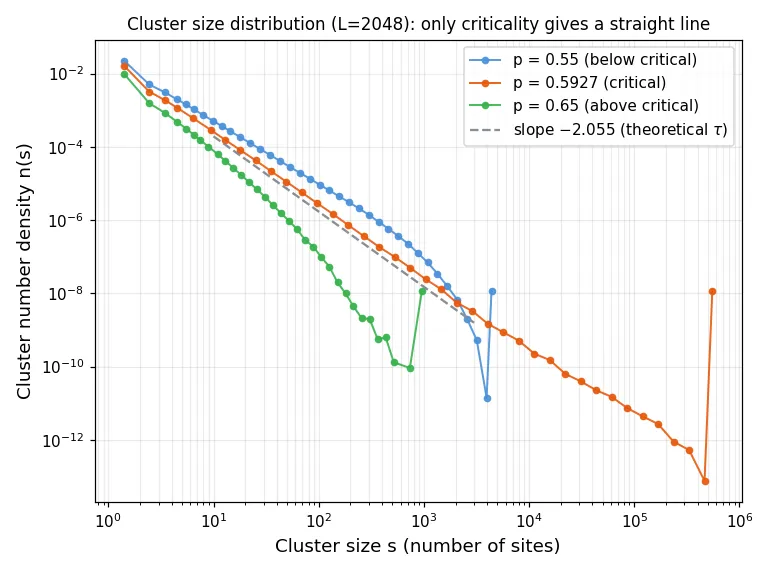
• At the critical point ($p=0.5927$): the distribution follows a straight line across five decades of size. The measured slope is $\tau = 2.00$ (theory is $187/91 \approx 2.055$). The fit residual is RMS 0.04 on a log scale — very nearly a perfect line
• Below critical ($p=0.55$): clusters larger than $s \approx 10^3$ die off exponentially. Fitting over the same range gives a residual of 0.49, an order of magnitude larger; it is not a straight line
• Above critical ($p=0.65$): removing the giant cluster leaves only fragments with $s < 10^3$, and the distribution bends away early, at $s \approx 10^2$ (residual 1.11)

The critical point is the only place with no characteristic size. Step off criticality and a bend always appears, a scale beyond which clusters essentially don’t exist. The straight line at the critical point means one and the same law governs everything from a cluster of size 1 to a monster of half a million sites.

Things worth stating honestly

• The scaling exponent of the transition width disagrees with theory. Measured $-0.83$ against a theoretical $-0.75$. Corrections to scaling are known to matter on small lattices like $L=64$, and the small-$L$ points are steepening the slope. I should refit using only larger lattices, but my compute budget stopped at $L=1024$
• $\tau = 2.00$ is also shallower than the theoretical 2.055. Finite size again: even at $L=2048$, the value moves by ±0.05 depending on how you choose the fit range. As with the Sierpiński dimension measurement, measuring a power-law exponent never escapes a negotiation with the fitting range
• The definition of spanning is somewhat arbitrary. I only looked top-to-bottom. Including left-right, or requiring both, shifts the finite-size curves slightly (the extrapolated infinite-size value doesn’t change)
• The fitted slope at $p=0.55$ came out at 2.05, coincidentally almost exactly the theoretical value. But look at the residual and it’s obvious the distribution is curved. A good lesson in not concluding “it follows a power law” from the exponent alone

What surprised me when I actually ran it

The biggest surprise was that finite-size effects showed up almost entirely in the width, not the position. Going in, I assumed a small lattice would put the transition point itself noticeably off. In fact even $L=64$ puts the 50%-spanning point at 0.5919, less than 0.001 from the true critical point. What was off was not the location but the spread: individual trials at $L=64$ run wild, spanning at 0.55 in one draw and refusing to span until 0.63 in another. “On average we already know the answer, but no individual answer is trustworthy” converges, as the lattice grows, into “every trial returns the same answer.”

The other surprise was how effective bisection is. Instead of sweeping $p$ finely and tracing out the spanning probability, you can pin down the exact $p$ at which each random field starts spanning with about a dozen cluster detections. If you want statistics on the transition point, measuring the $p_{\mathrm{span}}$ distribution directly beats measuring the S-curve by a wide margin. Where there’s monotonicity, there’s bisection.

And the strangeness of the critical landscape I genuinely did not anticipate until I saw the figure. Not below the transition, not above it, but at that one point, the system becomes “equally intricate at every scale you look.” So that is what a diverging correlation length looks like.

Criticality is a skeleton that applies to networks too, so it’s tempting to lay society over it. One or two extra connections change nothing, in almost every situation. But when the system happens to be near its critical point, that one connection becomes the bridge between continents. When something suddenly “spans” on social media, or the mood of an organization shifts from one day to the next, probably nothing big happened on the day it changed. The islands had been growing all along, and the last move happened to be a bridge. If that’s right, then a period with no visible change is not a period in which nothing is happening.

Reading the threshold and the percentages

The square-lattice, nearest-neighbor site-percolation threshold near 0.5927 is a numerical estimate, not an exact analytic value. See the Monte Carlo calculation by Newman and Ziff. The 0% and 100% reported here are fractions observed in 80 trials; they do not establish exact probabilities of zero or one on a finite lattice.

Summary

• Measured the spanning probability of 2D site percolation ($L \times L$ lattice, 4-neighbor) for $L = 64$ to $1024$
• The bigger the lattice, the steeper the transition: at $L=1024$, 1.5 percentage points of occupation (0.585 → 0.600) take the spanning probability from 0% to 100%
• The transition width shrinks as $L^{-0.83}$ (theory: $L^{-0.75}$); a 16-fold increase in $L$ shrinks it by roughly a factor of ten
• Extrapolating to an infinite lattice gives $p_c = 0.59249 \pm 0.00043$, agreeing with the established numerical estimate 0.59275 within 1σ
• The cluster size distribution follows the power law $n(s) \sim s^{-\tau}$ at the critical point and only there (measured $\tau = 2.00$, theory 2.055, straight across five decades); off criticality it bends at a characteristic scale
• Finite-size effects barely moved the location of the transition and showed up as its width — width dominated in this experiment, but finite-size estimates can also have a shifted transition location